Should I ask my data scientist about my medical condition?
It Depends
The above is half-joking, half-serious. The underlying notion is there exists a large intersection between data science and the life sciences.
Early in 2017, Kaggle, Intel, and MobileODT released a cervical cancer screening competition. The goal of the challenge was to identify which type of cervix was present given an image. In classifying cervix type correctly, doctors can prescribe the appropriate treatment for cancer, thus further mitigating future risk.
Cervical cancer is so easy to prevent if caught in its pre-cancerous stage that every woman should have access to effective, life-saving treatment no matter where they live. Today, women worldwide in low-resource settings are benefiting from programs where cancer is identified and treated in a single visit. However, due in part to lacking expertise in the field, one of the greatest challenges of these cervical cancer screen and treat programs is determining the appropriate method of treatment which can vary depending on patients’ physiological differences.
Especially in rural parts of the world, many women at high risk for cervical cancer are receiving treatment that will not work for them due to the position of their cervix. This is a tragedy: health providers are able to identify high risk patients, but may not have the skills to reliably discern which treatment which will prevent cancer in these women. Even worse, applying the wrong treatment has a high cost. A treatment which works effectively for one woman may obscure future cancerous growth in another woman, greatly increasing health risks.
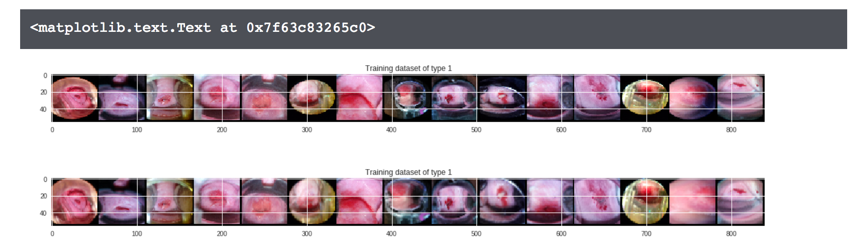
When looking at the data, one of the first things I noticed is that most of the photos had irrelevant information. For example, many either had black borders around the content or the instrument and other parts were present in the image. These additional object simply decrease the signal-to-noise ratio and thus convolute any predictions from a model learned from noisy data.
My idea was to create a smart crop in order to reduce the amount of irrelevant information learned from. Technically, with deep learning, we could supply more and more data combined with building bigger and bigger networks to perform the proper feature extraction, nullifying the bias-variance tradeoff. However, we don’t have that luxury here, though a good network should be able to extract a lot of relevant information. Of the higher-level features that can be constructed from the images, I believe the curvature yields the most information in predicting what type of cervix is in the image.
Knowing tools to use but not knowing how to perform proper image segmentation, I took to the web for insight. Coming from an ML-perspective, my initial thought was to use kmeans with K=2. This did reasonably well for a naive approach. However, the performance was very slow and some false positives were very wrong. In summary, what I tried was:
- Kmeans, K=2,3,4.
- Pros: Simple, correctly partitions some instances.
- Cons: Slow, doesn’t generalize well to multiple objects.
- Thesholding on hue (color).
- Pros: Simple, faster, performs well on well-curated images.
- Cons: Doesn’t perform well when other parts of the woman are in the image or when the signalling paste turns white.
- Creating all contours or edges (CV_CHAIN_APPROX_SIMPLE) with (CV_RETR_TREE) and without (CV_RETR_LIST) hierarchical structure.
- Pros: Granularity.
- Cons: Not straightforward how to make a useful crop, best combined as below.
- Finding contours with adaptive thresholding.
- Pros: null.
- Cons: Didn’t seem to partition any images well.
- Bounding boxes around contours.
- Pros: Extremely applicable, retains relevant information.
- Cons: Still retains some noise.
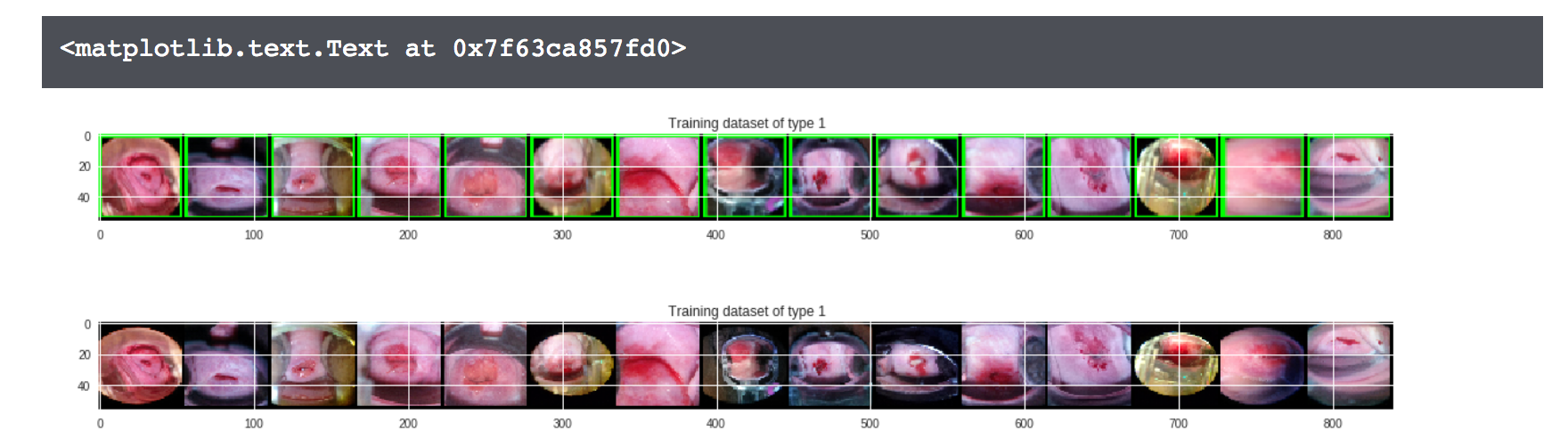
The main takeaway is the bounding boxes below, present in the latest Kaggle Kernel version. I found this to perform very well in that the crops were not aggressive so important information was not lost, while black borders and sometimes even other irrelevant parts were cropped. This intuitively increases the signal-to-noise ratio. A cherry on-top is that the crops are already rectangles, which can be exported to an image. With this Kaggle Kernel, I inspired several more kernels, being one of the first, if not the first, to post on creating a smart crop.
The solution I found to perform best:
def mask_black_bkgd(img):
    #Invert the image to be white on black for compatibility with findContours function.

    imgray = cv2.cvtColor(img, cv2.COLOR_BGR2GRAY)
    #Binarize the image and call it thresh.
    ret, thresh = cv2.threshold(imgray, 127, 255, cv2.THRESH_BINARY)

    #Find all the contours in thresh. In your case the 3 and the additional strike
    im2, contours, hierarchy = cv2.findContours(thresh, cv2.RETR_LIST, cv2.CHAIN_APPROX_SIMPLE)
    #Calculate bounding rectangles for each contour.
    rects = [cv2.boundingRect(cnt) for cnt in contours]

    #Calculate the combined bounding rectangle points.
    top_x = min([x for (x, y, w, h) in rects])
    top_y = min([y for (x, y, w, h) in rects])
    bottom_x = max([x+w for (x, y, w, h) in rects])
    bottom_y = max([y+h for (x, y, w, h) in rects])

    #Draw the rectangle on the image
    out = cv2.rectangle(img, (top_x, top_y), (bottom_x, bottom_y), (0, 255, 0), 2)
    crop = img[top_y:bottom_y,top_x:bottom_x]
    return crop #thresh
Produced via:
complete_images = []
for k, type_ids in enumerate([type_1_ids]): #, type_2_ids, type_3_ids]):
    m = int(np.floor(len(type_ids) / n))
    complete_image = np.zeros((m*(tile_size[0]+2), n*(tile_size[1]+2), 3), dtype=np.uint8)
    train_ids = sorted(type_ids)
    counter = 0
    for i in range(m):
        ys = i*(tile_size[1] + 2)
        ye = ys + tile_size[1]
        for j in range(n):
            xs = j*(tile_size[0] + 2)
            xe = xs + tile_size[0]
            image_id = train_ids[counter]; counter+=1
            img = get_image_data(image_id, 'Type_%i' % (k+1))
            img = cv2.resize(img, dsize=tile_size)
            #img = cv2.putText(img, image_id, (5,img.shape[0] - 5), cv2.FONT_HERSHEY_SIMPLEX, 2.0, (255, 255, 255), thickness=3)
            complete_image[ys:ye, xs:xe] = cv2.resize(mask_black_bkgd(img[:,:,:]), dsize=tile_size)
    complete_images.append(complete_image)

plt_st(20, 20)
plt.imshow(complete_images[0])
plt.title("Training dataset of type %i" % (1))
WARNING!! Images that some might find unsettling follow below. If you really don’t like to see gross images, now is your chance to turn back.
Cropped Images, with and without Bounding Boxes